Bayesian Statistics: The Science of Updating Beliefs with Data

The Mathematical Formula

Bayes' theorem, attributed to Reverend Thomas Bayes (1701-1761), provides the mathematical foundation for Bayesian statistics. The theorem states:

Where:

• P(θ|D) is the posterior probability of the parameters θ given the observed data D
• P(D|θ) is the likelihood of observing data D given parameters θ
• P(θ) is the prior probability of parameters θ before observing data
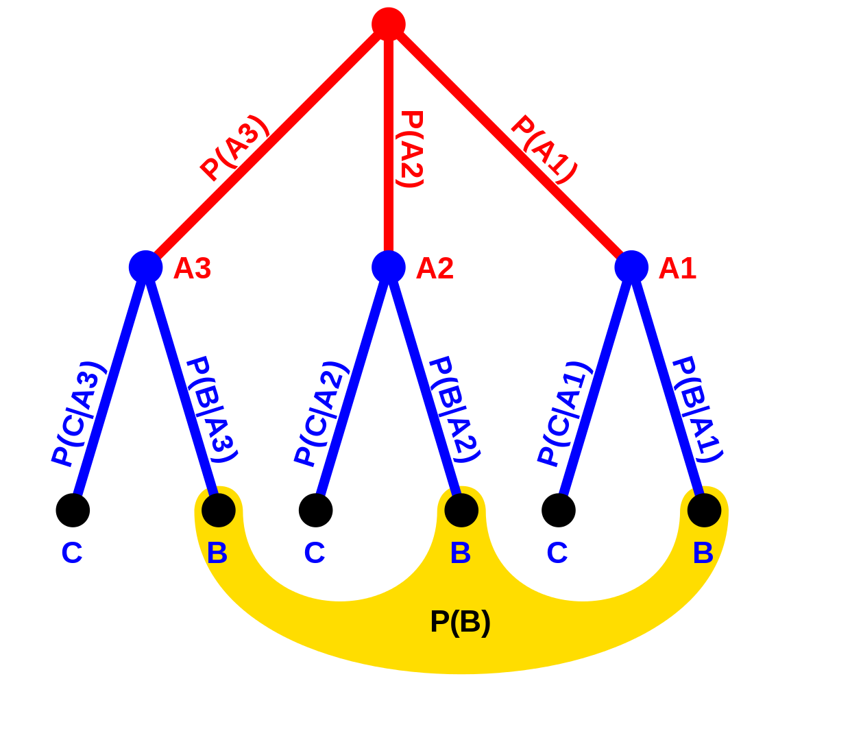
• P(D) is the marginal likelihood or evidence, calculated as the integral of the likelihood times the prior over all possible parameter values

A Simple Example

Consider testing for a disease that affects 1% of the population with a test that is 95% accurate (both sensitivity and specificity).

If a person tests positive, what is the probability they have the disease?

This classic example demonstrates the importance of accounting for both prior probabilities and likelihood ratios. Despite the test's high accuracy, the posterior probability of disease given a positive test is only about 16%, not 95% as many might intuitively guess. This illustrates how Bayesian reasoning can lead to counterintuitive but correct conclusions.

Types of Priors

• Informative Priors: Based on available information such as previous studies, expert opinion, or physical constraints. These priors express specific, substantive information about the parameters.
• Weakly Informative Priors: Provide some regularization and stability but don't dominate the posterior. They express general knowledge rather than specific information about parameters.
• Non-informative Priors: Designed to have minimal impact on the posterior, allowing the data to "speak for itself." Examples include uniform priors and Jeffreys' priors.
• Conjugate Priors: Priors that, when combined with certain likelihood functions, produce posteriors of the same distribution family. These are mathematically convenient and were especially important before modern computational methods.
• Hierarchical Priors: Priors that themselves depend on hyperparameters, which have their own prior distributions. These are useful for complex models and partial pooling of information across groups.

Common Prior Distributions

For different types of parameters, certain prior distributions are commonly used:

• For proportions: Beta distribution (conjugate to binomial likelihood)
• For means with known variance: Normal distribution (conjugate to normal likelihood)
• For variances: Inverse-Gamma or Half-Cauchy distributions
• For count parameters: Gamma or Poisson distributions
• For multivariate parameters: Multivariate normal, Wishart, or Dirichlet distributions

Definition and Properties

For a dataset D and parameter θ, the likelihood function L(θ; D) is proportional to the probability of observing D given θ:

Key properties of likelihood functions include:

• The likelihood is not a probability distribution over θ; it need not integrate to 1
• Only the relative values of the likelihood matter, not absolute values
• For independent observations, the likelihood is the product of individual observation likelihoods
• For computational reasons, we often work with the log-likelihood, which converts products to sums

Common Likelihood Functions

Different types of data require different likelihood functions:

• Binary outcomes: Bernoulli or binomial likelihood
• Count data: Poisson, negative binomial, or multinomial likelihood
• Continuous measurements: Normal, Student's t, or exponential likelihood
• Survival data: Exponential, Weibull, or Cox proportional hazards likelihood
• Categorical data: Multinomial or Dirichlet-multinomial likelihood

Interpretation and Usage

The posterior distribution P(θ|D) represents our complete state of knowledge about the parameters given the data. It allows us to:

• Calculate point estimates (mean, median, mode) of parameters
• Construct credible intervals to quantify parameter uncertainty
• Test hypotheses by calculating posterior probabilities
• Make predictions for future observations
• Perform decision analysis by integrating over parameter uncertainty

Posterior Summaries

Since the posterior is a probability distribution, we typically summarize it using:

• Point estimates:
  • Posterior mean: E[θ|D] - minimizes expected squared error
  • Posterior median: minimizes expected absolute error
  • Posterior mode (MAP estimate): maximizes posterior density
• Interval estimates:
  • Credible intervals: intervals containing a specified probability mass of the posterior
  • Highest posterior density (HPD) intervals: shortest intervals with specified probability
  • Equal-tailed intervals: equal probability in each tail
• Full distribution: For complex decisions or predictions, the entire posterior may be used

Markov Chain Monte Carlo (MCMC)

MCMC methods generate samples from the posterior distribution by constructing a Markov chain whose stationary distribution is the target posterior. Key MCMC algorithms include:

• Metropolis-Hastings: Proposes moves based on a proposal distribution and accepts or rejects them probabilistically based on the posterior ratios
• Gibbs Sampling: Updates one parameter at a time, sampling from its conditional posterior given all other parameters
• Hamiltonian Monte Carlo (HMC): Uses gradient information to propose more efficient moves, reducing random walk behavior and autocorrelation
• No-U-Turn Sampler (NUTS): An extension of HMC that automatically tunes the step size and number of steps

MCMC diagnostics are crucial to ensure the chain has:

• Converged to the stationary distribution (using multiple chains, Gelman-Rubin statistic)
• Explored the posterior space adequately (effective sample size, autocorrelation)
• Mixed well (trace plots, acceptance rates)

Variational Inference

Variational inference approximates the posterior with a simpler distribution (like a Gaussian) by minimizing the Kullback-Leibler divergence between the approximation and the true posterior. It is typically faster than MCMC but may be less accurate, especially for complex, multimodal posteriors.

Methods include:

• Mean-field variational inference: Assumes independence between parameters in the approximating distribution
• Stochastic variational inference: Uses stochastic optimization for large datasets
• Automatic differentiation variational inference (ADVI): Automatically transforms constrained variables and uses automatic differentiation for optimization

Bayesian Model Comparison

The key quantities for Bayesian model comparison are:

• Marginal likelihood (evidence): P(D|M) = ∫ P(D|θ,M) × P(θ|M) dθ, the probability of the data under a given model, integrating over all parameter values
• Bayes factors: The ratio of marginal likelihoods for two competing models, measuring the relative evidence they provide
• Posterior model probabilities: P(M|D) ∝ P(D|M) × P(M), the probability of each model given the data and prior model probabilities

Information Criteria

When the marginal likelihood is difficult to compute, various information criteria can be used as approximations:

• Deviance Information Criterion (DIC): Particularly useful for hierarchical models and MCMC outputs
• Widely Applicable Information Criterion (WAIC): A fully Bayesian approach that uses the entire posterior distribution
• Leave-One-Out Cross-Validation (LOO-CV): Estimates out-of-sample predictive accuracy
• Bayesian Information Criterion (BIC): An asymptotic approximation to the log marginal likelihood

Data Science and Machine Learning

• Bayesian Neural Networks: Add uncertainty quantification to neural network predictions
• Gaussian Processes: Flexible non-parametric models for regression and classification
• Bayesian Optimization: Efficient exploration of parameter spaces for hyperparameter tuning
• Topic Models: Latent Dirichlet Allocation and other Bayesian methods for document analysis
• Causal Inference: Bayesian networks and structural equation models for causal relationships

Science and Research

• Clinical Trials: Adaptive designs, benefit-risk assessment, and subgroup analysis
• Genomics: Gene expression analysis, genome-wide association studies
• Ecology: Species distribution models, capture-recapture studies, population dynamics
• Astronomy: Image processing, cosmological parameter estimation
• Climate Science: Climate model calibration, paleoclimate reconstruction

Business and Economics

• Marketing: Customer behavior modeling, A/B testing, marketing mix models
• Finance: Portfolio optimization, risk assessment, option pricing
• Econometrics: Time series forecasting, causal impact analysis
• Supply Chain: Demand forecasting, inventory optimization
• Pricing: Dynamic pricing strategies, elasticity estimation

References

- Gelman, Carlin, Stern, Dunson, Vehtari, and Rubin. Bayesian Data Analysis. 2013.
- McElreath. Statistical Rethinking: A Bayesian Course with Examples in R and Stan. 2020.
Last reviewed: April 15, 2026
Maintained by MathCalculate Editorial as part of the public quantitative reference library.
Key topics covered: This article explores bayesian statistics, bayesian inference, prior distribution, posterior distribution, bayes theorem, probabilistic modeling, bayesian computational methods, and mcmc, together with real-world applications.