Linear Regression: Principles, Methods and Applications

Introduction to Linear Regression

Linear regression is one of the most fundamental and widely used statistical methods for modeling the relationship between a dependent variable and one or more independent variables. It serves as the cornerstone of statistical learning, providing a simple yet powerful framework for both prediction and inference.

At its core, linear regression attempts to model the relationship by fitting a linear equation to observed data. The simplicity of the linear model, combined with its interpretability and computational efficiency, has made it an indispensable tool across diverse fields including economics, biology, social sciences, engineering, and machine learning.

Whether used to identify causal relationships, make predictions, or understand the strength of associations between variables, linear regression provides a versatile analytical approach with strong theoretical foundations and practical applications in data analysis and scientific research.

Mathematical Foundations

The mathematical foundations of linear regression provide a rigorous framework for understanding how the model works and what assumptions underlie its application.

Simple Linear Regression

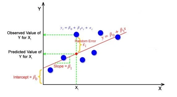
In simple linear regression, we model the relationship between two variables: a dependent variable y and an independent variable x. The model is described by the equation:

where:

• y is the dependent (or response) variable
• x is the independent (or predictor) variable
• β₀ is the intercept (value of y when x = 0)
• β₁ is the slope (change in y for a unit change in x)
• ε is the error term, representing random noise and unmodeled factors

Multiple Linear Regression

Multiple linear regression extends the simple model to include multiple independent variables:

This can be more compactly written in matrix notation as:

where:

• y is an n×1 vector of responses for n observations
• X is an n×(p+1) matrix of predictors (including a column of 1s for the intercept)
• β is a (p+1)×1 vector of regression coefficients
• ε is an n×1 vector of error terms

Model Assumptions

The classical linear regression model makes several key assumptions:

1. Linearity: The relationship between the dependent and independent variables is linear
2. Independence: The observations are independent of each other
3. Homoscedasticity: The error terms have constant variance (Var(ε) = σ²)
4. Normality: The error terms are normally distributed (ε ~ N(0, σ²))
5. No multicollinearity: The independent variables are not perfectly correlated with each other

Violations of these assumptions can lead to biased or inefficient parameter estimates and invalid standard errors, potentially undermining the reliability of inference and predictions.

Estimation Methods

The primary goal in linear regression is to estimate the unknown parameters (coefficients) of the model. Several methods exist for this purpose, each with its own theoretical foundations and practical considerations.

Ordinary Least Squares (OLS)

The most common method for estimating linear regression parameters is Ordinary Least Squares (OLS). OLS minimizes the sum of squared residuals between the observed responses and the predictions:

In matrix form, the OLS estimator for β is:

where X' denotes the transpose of X.

OLS estimators have several desirable properties when the assumptions of the classical linear model are met:

• Unbiasedness: E[β̂] = β, meaning the expected value of the estimator equals the true parameter value
• Efficiency: Among all unbiased linear estimators, OLS has the smallest variance (Gauss-Markov theorem)
• Consistency: As the sample size increases, the estimator converges in probability to the true parameter value
• Normality: Under the assumption of normal errors, the OLS estimators are also normally distributed

Maximum Likelihood Estimation (MLE)

Another approach to parameter estimation is Maximum Likelihood Estimation, which finds the parameter values that maximize the likelihood of observing the given data.

For linear regression with normally distributed errors, the MLE and OLS estimators coincide. However, MLE provides a more general framework that can be extended to other error distributions and more complex models.

Bayesian Estimation

Bayesian approaches to linear regression incorporate prior beliefs about the parameters and update these beliefs using observed data. The result is a posterior distribution of the parameters rather than point estimates, providing a natural framework for quantifying uncertainty in parameter estimates and predictions.

Statistical Inference and Prediction

Linear regression serves dual purposes: inference about relationships between variables and prediction of new observations.

Inference on Coefficients

Once we have estimated the regression coefficients, we often want to conduct statistical inference, such as testing hypotheses and constructing confidence intervals.

Under the classical assumptions, the OLS estimator β̂ follows a normal distribution:

This allows us to:

• Test hypotheses: H₀: βⱼ = 0 vs. H₁: βⱼ ≠ 0 using t-tests
• Construct confidence intervals: β̂ⱼ ± t₍α/2,n-p-1₎·SE(β̂ⱼ)
• Test joint hypotheses: Using F-tests for multiple constraints on the coefficients

Prediction

Linear regression models can be used to make predictions for new observations. For a given set of predictor values x₀, the predicted response is:

There are two types of prediction intervals:

• Confidence interval for the mean response: Quantifies uncertainty in the estimated mean response at x₀
• Prediction interval for an individual observation: Accounts for both the uncertainty in the estimated mean response and the random variation around the mean

Model Evaluation

Several metrics help evaluate the performance of linear regression models:

• Coefficient of Determination (R²): Proportion of variance in the dependent variable explained by the model, ranging from 0 to 1
• Adjusted R²: Modified version that accounts for the number of predictors, useful for comparing models of different complexity
• Root Mean Squared Error (RMSE): Square root of the average squared prediction error
• Mean Absolute Error (MAE): Average absolute prediction error
• Akaike Information Criterion (AIC): Balances model fit and complexity for model selection

Regression Diagnostics

Regression diagnostics help assess whether the model assumptions are satisfied and identify potentially problematic observations.

Residual Analysis

Residuals (eᵢ = yᵢ - ŷᵢ) provide valuable insights into model fit:

• Residual plots: Plotting residuals against fitted values or predictors can reveal patterns indicating non-linearity or heteroscedasticity
• Normal probability plots: Assess whether residuals follow a normal distribution
• Residual autocorrelation: Tests like Durbin-Watson detect temporal or spatial correlation in residuals

Influential Observations

Some observations can have disproportionate influence on the regression results:

• Leverage: Measures the potential influence of an observation based on its predictor values
• Cook's distance: Quantifies the overall influence of an observation on both predictions and coefficient estimates
• DFBETAS: Measures the change in coefficient estimates when an observation is excluded
• Studentized residuals: Standardized residuals that account for their varying precision

Common Violations and Remedies

When assumptions are violated, several remedies are available:

• Non-linearity: Transform variables, add polynomial terms, or use nonparametric regression
• Heteroscedasticity: Use weighted least squares or robust standard errors
• Non-normality: Transform the response variable or use robust regression
• Multicollinearity: Remove redundant predictors, use regularization, or principal component regression
• Autocorrelation: Use generalized least squares or time series models

Regularization and Shrinkage Methods

When dealing with many predictors or multicollinearity, regularization methods can improve prediction accuracy and model interpretability by shrinking or constraining the regression coefficients.

Ridge Regression

Ridge regression adds a penalty on the sum of squared coefficients:

where λ > 0 is a tuning parameter that controls the amount of shrinkage. As λ increases, the coefficients are increasingly shrunk toward zero, but typically not exactly to zero.

Ridge regression is particularly useful when predictors are highly correlated, as it stabilizes the coefficient estimates by reducing their variance, albeit at the cost of introducing some bias.

Lasso Regression

Lasso (Least Absolute Shrinkage and Selection Operator) uses a penalty on the sum of absolute coefficient values:

Unlike ridge regression, lasso can shrink some coefficients exactly to zero, effectively performing variable selection. This makes lasso particularly valuable when dealing with a large number of predictors, many of which may be irrelevant.

Elastic Net

Elastic Net combines the ridge and lasso penalties:

Elastic Net inherits the variable selection property of lasso while maintaining ridge's ability to handle correlated predictors. It's particularly useful when the number of predictors exceeds the number of observations.

Extensions and Variants

The basic linear regression model has been extended in numerous ways to accommodate various types of data and modeling scenarios.

Polynomial Regression

Polynomial regression extends linear regression by including polynomial terms of the predictors:

This allows modeling nonlinear relationships while still using the linear regression framework, as the model remains linear in the parameters.

Robust Regression

Robust regression methods provide resistance to outliers and violations of assumptions:

• M-estimation: Minimizes a function of residuals that is less sensitive to large residuals than squared loss
• Least Absolute Deviations (LAD): Minimizes the sum of absolute residuals
• Huber loss: Combines squared loss for small residuals and absolute loss for large residuals

Weighted Least Squares

Weighted least squares accounts for heteroscedasticity by assigning different weights to observations:

Observations with higher variance receive lower weights, leading to more efficient parameter estimates when the variance structure is correctly specified.

Generalized Linear Models (GLMs)

GLMs extend linear regression to handle non-normal response distributions and non-linear relationships through a link function:

Examples include:

• Logistic regression: For binary responses, using a logit link
• Poisson regression: For count data, using a log link
• Gamma regression: For positive continuous data, often using a log or inverse link

Panel Data Models

For data with both cross-sectional and temporal dimensions, panel data models incorporate individual-specific and time-specific effects:

• Fixed effects: Accounts for time-invariant unobserved heterogeneity
• Random effects: Treats individual effects as random variables
• Dynamic panel models: Includes lagged dependent variables as predictors

Applications

Linear regression has found widespread applications across various domains, demonstrating its versatility and utility.

Economics and Finance

Econometric modeling: Linear regression is the foundation of econometrics, used to estimate relationships between economic variables, test economic theories, and make forecasts.

Financial applications: Regression models help analyze asset returns, measure systematic risk (beta), and evaluate portfolio performance through models like the Capital Asset Pricing Model (CAPM).

Biostatistics and Medical Research

Epidemiology: Regression models help identify risk factors for diseases by examining associations between exposures and health outcomes.

Clinical trials: Linear models are used to analyze treatment effects while adjusting for covariates.

Social Sciences

Psychology: Regression helps investigate relationships between psychological constructs and behaviors.

Sociology: Linear models examine how social factors influence outcomes like education, income, or health.

Machine Learning and Predictive Analytics

Predictive modeling: Despite the development of more complex algorithms, linear regression remains a benchmark model and is often surprisingly competitive in predictive tasks.

Feature importance: Regression coefficients provide insights into which features are most important for prediction.

Environmental Sciences

Climate modeling: Regression models help analyze relationships between climate variables and identify trends.

Ecological studies: Linear models examine how environmental factors affect species distribution and abundance.

Limitations and Considerations

Despite its versatility, linear regression has limitations that should be considered in its application.

Conceptual Limitations

Causality: Regression identifies associations but does not necessarily imply causation. Confounding variables, reverse causality, and selection bias can all lead to misleading conclusions if regression results are interpreted causally without appropriate research design.

Linear relationships: The model assumes linear relationships between predictors and the response, which may not capture complex, nonlinear patterns in the data.

Statistical Limitations

Sensitivity to outliers: OLS estimates can be heavily influenced by extreme observations, potentially leading to distorted coefficient estimates.

Multicollinearity: When predictors are highly correlated, coefficient estimates become unstable and difficult to interpret individually.

Omitted variable bias: Excluding relevant predictors can lead to biased coefficient estimates for the included variables.

Practical Considerations

Data quality: Linear regression assumes accurate measurement of variables, with errors in predictors potentially leading to attenuation bias.

Sample size: Small samples may not provide enough statistical power to detect relationships or may lead to overfitting, especially with many predictors.

Prediction limits: Extrapolating beyond the range of observed data can lead to unreliable predictions, as the linear relationship may not hold in unexplored regions.

Computational Implementation

Modern computational tools make linear regression accessible and efficient to implement.

Matrix Computation

For moderate-sized datasets, linear regression can be efficiently implemented using direct matrix operations:

Numerically stable implementations often use QR decomposition or Singular Value Decomposition (SVD) rather than directly computing the inverse of X'X.

Iterative Methods

For large datasets, iterative optimization algorithms are often used:

• Gradient Descent: Updates parameters in the direction of steepest decrease in the cost function
• Stochastic Gradient Descent: Uses random subsets of data for each update, making it suitable for very large datasets
• Coordinate Descent: Updates one parameter at a time, particularly efficient for regularized regression

Software Implementation

Linear regression is implemented in virtually all statistical and machine learning software:

• R: The lm() function for basic linear regression, with packages like glmnet for regularized regression
• Python: scikit-learn provides LinearRegression, Ridge, Lasso, and other variants
• MATLAB/Octave: Functions like regress and fitlm
• SAS: PROC REG and PROC GLM for various regression models

Conclusion

Linear regression stands as one of the most fundamental methods in statistical analysis and machine learning, serving as both a practical tool for data analysis and a conceptual building block for more complex methods.

Its mathematical elegance, computational simplicity, and interpretability make it a cornerstone of quantitative research across disciplines. When used appropriately—with careful attention to assumptions, diagnostics, and limitations—linear regression provides a powerful framework for understanding relationships between variables and making predictions.

The extensions and variants of linear regression, from ridge and lasso to generalized linear models, further expand its utility, allowing it to address a wide range of data structures and modeling challenges.

As data science continues to evolve, linear regression remains a fundamental tool in the data analyst's toolkit, providing a benchmark against which more complex models are compared and a foundation upon which more sophisticated methods are built.

References

- Montgomery, Peck, and Vining. Introduction to Linear Regression Analysis. 2021.
- Kutner, Nachtsheim, Neter, and Li. Applied Linear Statistical Models. 2004.
Last reviewed: April 15, 2026
Maintained by MathCalculate Editorial as part of the public quantitative reference library.
Key topics covered: This article explores linear regression, ordinary least squares, regression analysis, statistical modeling, coefficient of determination, multivariate regression, statistical inference, and residual analysis, together with real-world applications.