Normal Distribution: The Bell Curve Explained

What is the Normal Distribution?

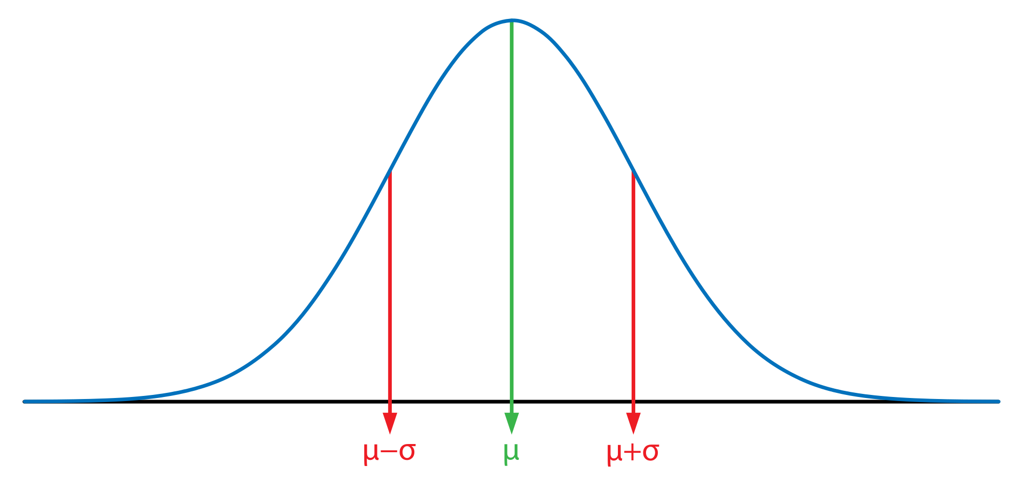
The normal distribution, also known as the Gaussian distribution or bell curve, is a continuous probability distribution that is symmetrically distributed around its mean. It is one of the most important probability distributions in statistics because many natural phenomena follow this pattern.

A normal distribution is characterized by two parameters:

Mean (μ): The central value or average, which determines the location of the peak
Standard deviation (σ): A measure of dispersion that determines the width or spread of the distribution

The probability density function (PDF) of a normal distribution is given by:

f(x) = (1 / (σ√(2π))) * e^(-(x-μ)²/(2σ²))

This seemingly complex formula produces the iconic bell-shaped curve that has become synonymous with statistical normality and has profound applications across many disciplines, from natural sciences to finance and quality control.

Historical Background and Discovery

The normal distribution has a rich and fascinating history spanning several centuries of mathematical development:

Origins in Error Analysis

The concept of the normal distribution emerged in the 18th century from the study of errors in astronomical and geodetic measurements. Scientists needed a mathematical model to understand the distribution of measurement errors.

Abraham de Moivre, a French mathematician, first introduced what we now call the normal distribution in 1733. In his work on probability, he derived the mathematical formula while solving problems related to the binomial distribution. However, his discovery remained relatively obscure for decades.

Gauss and the Method of Least Squares

Carl Friedrich Gauss, the renowned German mathematician, made significant contributions to the development of the normal distribution in the early 19th century. While analyzing astronomical data, Gauss formalized the distribution's properties and derived the method of least squares, which is used to find the best fit for data with random errors. His work was so influential that the normal distribution is often called the "Gaussian distribution" in his honor.

Gauss published his work on the normal distribution in his 1809 treatise "Theoria Motus Corporum Coelestium" (Theory of the Motion of Celestial Bodies), where he demonstrated that measurement errors followed this distribution pattern.

Laplace and the Central Limit Theorem

Pierre-Simon Laplace, a French mathematician and astronomer, independently worked on the normal distribution around the same time as Gauss. In 1810, Laplace published his work on probability theory, which included early formulations of what would later become known as the Central Limit Theorem a fundamental concept explaining why many natural phenomena follow a normal distribution.

Modern Significance

By the late 19th century, the normal distribution had become a cornerstone of statistical theory. Francis Galton's work on regression and correlation, along with Karl Pearson's development of mathematical statistics, further solidified the importance of the normal distribution.

Today, the normal distribution remains one of the most widely used probability distributions in statistical analysis, with applications ranging from natural sciences and engineering to finance, medicine, and social sciences.

Key Properties and Characteristics

Shape and Symmetry

The normal distribution has several distinctive properties that make it mathematically elegant and practically useful:

Symmetry: The distribution is perfectly symmetrical around its mean (μ), which is also its mode and median
Bell shape: The characteristic "bell curve" shape has a single peak at the mean and tapers off in both directions
Asymptotic tails: The tails of the distribution extend infinitely in both directions, approaching but never touching the x-axis
Inflection points: The curve changes from concave down to concave up (or vice versa) at μ ± σ

The 68-95-99.7 Rule

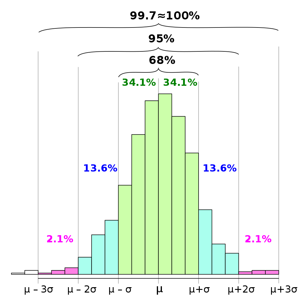
One of the most practical features of the normal distribution is the "empirical rule" or "68-95-99.7 rule":

68% of observations fall within 1 standard deviation of the mean (μ ± σ)
95% of observations fall within 2 standard deviations of the mean (μ ± 2σ)
99.7% of observations fall within 3 standard deviations of the mean (μ ± 3σ)

This rule provides a quick and practical way to interpret normal distribution data without complex calculations.

Standard Normal Distribution

The standard normal distribution is a special case where μ = 0 and σ = 1. It is denoted by Z and serves as a reference distribution:

f(z) = (1/√(2π)) * e^(-z²/2)

Any normal random variable X can be transformed into a standard normal random variable Z using the formula:

Z = (X - μ) / σ

This process, known as standardization or z-transformation, allows us to use standardized tables and simplify probability calculations.

Mathematical Properties

Expected value: E[X] = μ (The expected value equals the mean)
Variance: Var(X) = σ² (The variance equals the square of the standard deviation)
Skewness: 0 (The distribution is perfectly symmetric with no skew)
Kurtosis: 3 (Standard measure of "tailedness" for normal distribution)
Entropy: (1/2) * ln(2πeσ²) (Measures the uncertainty or randomness)
Moment-generating function: M(t) = exp(μt + σ²t²/2)

The Central Limit Theorem

The Central Limit Theorem (CLT) is one of the most important concepts in probability theory and helps explain why the normal distribution is so prevalent in nature.

The Fundamental Principle

The Central Limit Theorem states that when you take a large number of independent random samples from any distribution (with finite mean and variance), the distribution of sample means will approximate a normal distribution, regardless of the original distribution's shape.

More formally, if X₁, X₂, ..., Xₙ are independent and identically distributed random variables with mean μ and standard deviation σ, then as n increases, the distribution of the sample mean approaches a normal distribution with mean μ and standard deviation σ/√n.

Practical Implications

The Central Limit Theorem has profound implications for statistical inference and data analysis:

Statistical inference: It allows us to make inferences about population parameters using sample statistics, even when the population distribution is unknown or non-normal
Sample size considerations: Generally, sample sizes of 30 or more are considered sufficient for the CLT to apply, though this can vary depending on how far the original distribution deviates from normality
Confidence intervals: The CLT enables the construction of confidence intervals around sample estimates
Hypothesis testing: Many statistical tests rely on the CLT to justify the assumption of normally distributed test statistics

Why Natural Phenomena Often Follow Normal Distributions

The Central Limit Theorem helps explain why so many natural phenomena exhibit normal distributions. Many natural measurements are actually the sum or average of numerous small, independent random factors. For example:

Human height: Influenced by many independent genetic and environmental factors
Measurement errors: Result from many small, independent sources of error
Biological measurements: Often represent the cumulative effect of many small biological processes
Test scores: Reflect the combined influence of many factors affecting performance

Real-World Applications

Natural Sciences

Physics: Describes the distribution of particles in gases (kinetic theory), random motion in diffusion processes, and thermal noise in electronic systems
Biology: Models variations in physical traits across populations, such as height, weight, or blood pressure
Medicine: Used in analyzing lab test results, determining reference ranges for medical tests, and evaluating the effectiveness of treatments
Environmental science: Models pollution dispersion, rainfall patterns, and other environmental measurements

Business and Finance

Risk management: Models financial risks and potential investment returns through the normal distribution
Black-Scholes model: Uses normal distribution assumptions for option pricing in financial markets
Portfolio theory: Utilizes normal distribution to model portfolio returns and optimize asset allocation
Actuarial science: Models insurance claims and establishes premium rates

Quality Control and Manufacturing

Six Sigma: A data-driven methodology that uses normal distribution principles to improve manufacturing processes by reducing defects
Statistical process control: Uses normal distribution to monitor production processes and detect abnormalities
Tolerance analysis: Ensures that parts will fit together in assembly by accounting for normal variations in manufacturing
Acceptance sampling: Determines whether to accept or reject a batch of products based on sample statistics

Social Sciences and Education

Standardized testing: Test scores are often designed to follow a normal distribution, with methods like curve grading
Psychology: Used to interpret psychological test results and understand the distribution of traits in populations
Economics: Models income distribution, consumption patterns, and economic forecasts
Demographic studies: Analyzes population characteristics and their distributions

Calculating and Working with Normal Distributions

Finding Probabilities

To find the probability that a normally distributed random variable X falls within a particular range [a, b]:

P(a ≤ X ≤ b) = Φ((b-μ)/σ) - Φ((a-μ)/σ)

Where Φ is the cumulative distribution function (CDF) of the standard normal distribution.

For the standard normal distribution, values of Φ(z) are widely available in statistical tables or can be calculated using software.

Z-Score Calculation

The Z-score indicates how many standard deviations an observation is from the mean:

Z = (X - μ) / σ

A positive Z-score indicates the observation is above the mean, while a negative Z-score indicates it's below the mean.

Z-scores are particularly useful for:

Comparing observations from different distributions: Z-scores standardize values to a common scale
Identifying outliers: Observations with |Z| > 3 are often considered outliers
Creating percentiles: Z-scores can be converted to percentiles using standard normal tables

Implementation in JavaScript

Here's a JavaScript implementation for calculating normal distribution probabilities:

// Standard Normal cumulative distribution function
function standardNormalCDF(z) {
  // Approximation using error function
  return 0.5 * (1 + erf(z / Math.sqrt(2)));
}

// Error function approximation
function erf(x) {
  // Constants
  const a1 =  0.254829592;
  const a2 = -0.284496736;
  const a3 =  1.421413741;
  const a4 = -1.453152027;
  const a5 =  1.061405429;
  const p  =  0.3275911;

  // Save the sign
  const sign = (x < 0) ? -1 : 1;
  x = Math.abs(x);

  // Formula
  const t = 1.0 / (1.0 + p * x);
  const y = 1.0 - (((((a5 * t + a4) * t) + a3) * t + a2) * t + a1) * t * Math.exp(-x * x);

  return sign * y;
}

// Normal distribution probability: P(a ≤ X ≤ b) where X ~ N(mean, stdDev)
function normalProbability(a, b, mean, stdDev) {
  const za = (a - mean) / stdDev;
  const zb = (b - mean) / stdDev;
  return standardNormalCDF(zb) - standardNormalCDF(za);
}

// Normal distribution PDF
function normalPDF(x, mean, stdDev) {
  return (1 / (stdDev * Math.sqrt(2 * Math.PI))) * 
         Math.exp(-0.5 * Math.pow((x - mean) / stdDev, 2));
}

Common Misconceptions

All data are normally distributed: While many natural phenomena follow normal distributions, many do not. Examples of non-normal distributions include income distributions (often right-skewed) and reaction times (often not symmetric).
Normal distributions have no outliers: While extreme values are increasingly rare, the normal distribution extends infinitely in both directions, allowing for the possibility of extreme values.
Small samples from non-normal populations follow normal distributions: The Central Limit Theorem applies to sample means, not to individual observations or very small samples.
Statistical tests always require normality: While many tests assume normality, some are robust against deviations from normality, and others are specifically designed for non-normal data.

Last Updated: March 12, 2025

Keywords: normal distribution, bell curve, gaussian distribution, standard normal distribution, probability density function, statistics, central limit theorem, z-score, statistical inference, quantitative methods, data analysis, probability theory, empirical rule, variance, standard deviation, cumulative distribution function

References

- Gauss. Theoria Motus Corporum Coelestium in Sectionibus Conicis Solem Ambientium. 1809.
- Fisher. Statistical Methods for Research Workers. 1925.
Last reviewed: April 15, 2026
Maintained by MathCalculate Editorial as part of the public quantitative reference library.
Key topics covered: This article explores normal distribution, bell curve, gaussian distribution, standard normal distribution, probability density function, statistics, central limit theorem, and z-score, together with real-world applications.